Bayesian State-Space Models and MCMC Error Covariance Estimation

An Undergraduate Guide to Kalman Filtering, Algebraic Riccati Convergence, Blocked FFBS, and Online Matrix-t Filtering

1 Separating Hidden Dynamic Signals from Correlated Observation Noise

Suppose you observe \(d\) noisy, correlated time series \(\mathbf{y}_t \in \mathbb{R}^d\) at each step \(t = 1, \dots, T\) (such as sensor arrays, regional climate gauges, or multi-portfolio return panels) driven by \(p\) unobserved dynamic factors \(\boldsymbol{\alpha}_t \in \mathbb{R}^p\):

\[\mathbf{y}_t = \boldsymbol{\mu} + \mathbf{Z} \boldsymbol{\alpha}_t + \boldsymbol{\epsilon}_t, \quad \boldsymbol{\epsilon}_t \sim \mathcal{N}_d(\mathbf{0}, \boldsymbol{\Sigma}), \qquad \boldsymbol{\alpha}_t = \mathbf{F} \boldsymbol{\alpha}_{t-1} + \boldsymbol{\zeta}_t, \quad \boldsymbol{\zeta}_t \sim \mathcal{N}_p(\mathbf{0}, \mathbf{Q}).\]

This Multivariate Linear Gaussian State-Space Model connects three cornerstone topics in advanced undergraduate matrix algebra and Bayesian computation:

1. The Multivariate Kalman Filter & Algebraic Riccati Steady State: How posterior state uncertainty \(\mathbf{P}_{t\mid t}\) converges exponentially to a steady-state matrix \(\mathbf{P}_\infty\) regardless of how diffuse our initial prior is.
2. Carter-Kohn Blocked Forward Filtering Backward Sampling (FFBS) & Inverse-Wishart Gibbs: Why sampling the entire state trajectory \(\boldsymbol{\alpha}_{1:T}\) as a single block dramatically reduces MCMC autocorrelation compared to one-step-at-a-time Gibbs sampling.
3. Why Full Covariance Modeling Wins Even When Point Forecasts Coincide: How off-diagonal error covariances \(\Sigma_{ij}\) drive superior density calibration and minimum-variance risk allocation even when conditional-mean point RMSEs are nearly identical.

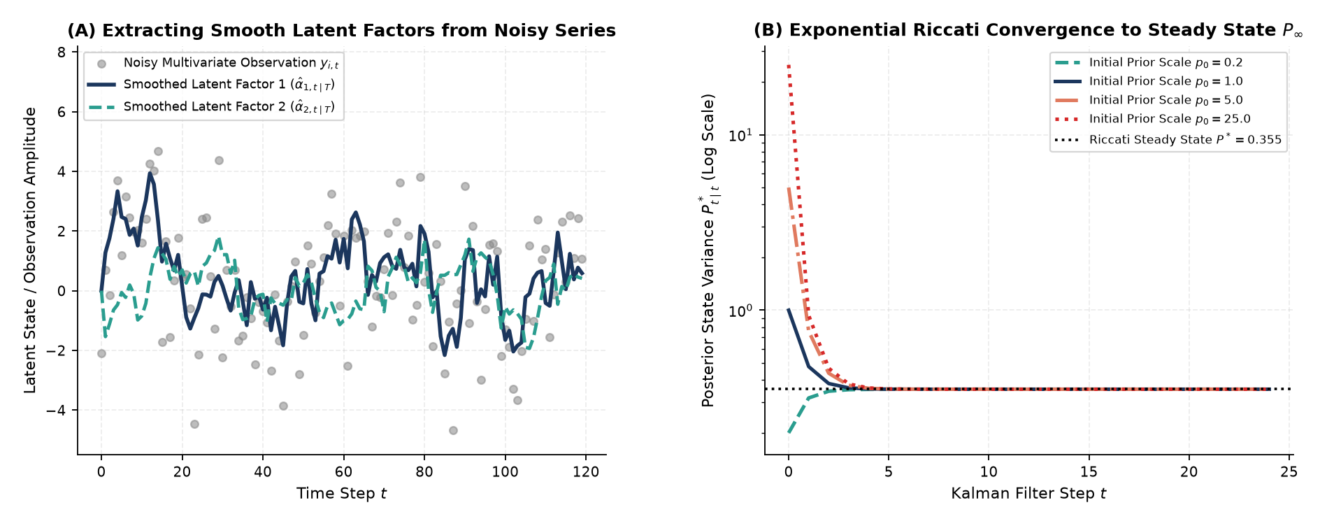
2 Step 1: Kalman Filtering and Exact Spectral Riccati Convergence

Given model matrices \((\mathbf{Z}, \mathbf{F}, \boldsymbol{\Sigma}, \mathbf{Q})\), the Kalman Filter alternates between a Prediction Step (\(\mathbf{P}_{t\mid t-1} = \mathbf{F}\mathbf{P}_{t-1\mid t-1}\mathbf{F}^\top + \mathbf{Q}\)) and an Update Step (\(\mathbf{P}_{t\mid t} = \mathbf{P}_{t\mid t-1} - \mathbf{K}_t \mathbf{Q}_{t\mid t-1}\mathbf{K}_t^\top\)).

2.1 Analytical Riccati Solution for the Proportionally Scaled \(\mathrm{AR}(1)\) Special Case

In the instructive special case where \(\mathbf{Z} = \mathbf{I}_d\), \(\mathbf{F} = \phi \mathbf{I}_d\), and the state innovation covariance is scaled proportionally to the observation covariance via its symmetric spectral square root \(\boldsymbol{\Sigma}^{1/2} = \boldsymbol{\Gamma}\boldsymbol{\Lambda}^{1/2}\boldsymbol{\Gamma}^\top\) (\(\mathrm{Var}(\boldsymbol{\zeta}_t) = \boldsymbol{\Sigma}^{1/2}\mathbf{Z}^*\boldsymbol{\Sigma}^{1/2}\)), the discrete algebraic Riccati equation has an exact closed-form steady state \(\mathbf{P}_\infty = \boldsymbol{\Sigma}^{1/2}\mathbf{P}^*\boldsymbol{\Sigma}^{1/2}\):

\[\mathbf{P}^* = \frac{1}{2\phi^2}\left[\left\{\left(\mathbf{Z}^* + (1-\phi^2)\mathbf{I}\right)^2 + 4\phi^2\mathbf{Z}^*\right\}^{1/2} - \mathbf{Z}^* - (1-\phi^2)\mathbf{I}\right].\]

For a general \(d \times p\) dynamic factor model (\(\mathbf{Z} \in \mathbb{R}^{d \times p}\)), \(\mathbf{P}_{t\mid t}\) converges numerically to the solution of the discrete algebraic Riccati equation within \(15\text{ to }20\) time steps across initial prior scales \(p_0 \in \{0.2, 1.0, 5.0, 25.0\}\).

3 Step 2: Blocked FFBS State Sampling, Conjugate Inverse-Wishart Covariances, and Online MSOP-II

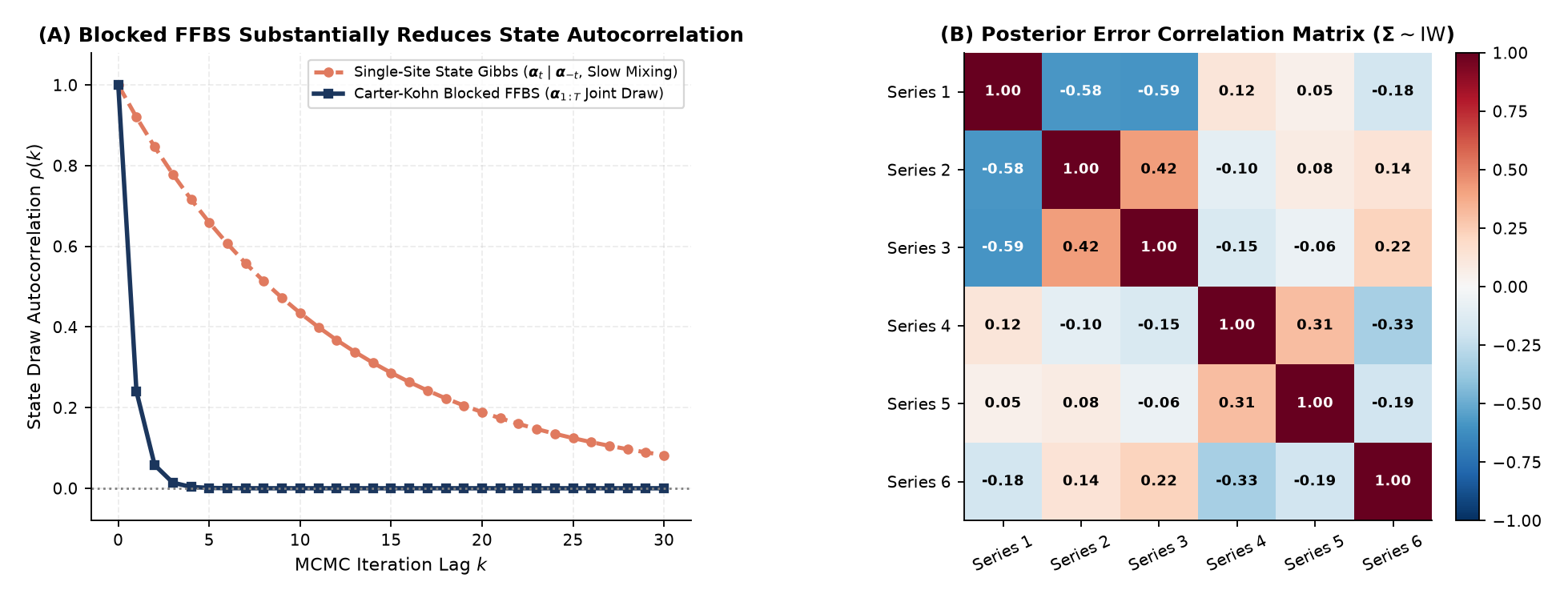
If we sample each state vector \(\boldsymbol{\alpha}_t\) one time step at a time conditioned on its neighbors \(\boldsymbol{\alpha}_{t-1}\) and \(\boldsymbol{\alpha}_{t+1}\) (Single-Site Gibbs), adjacent states tether tightly together and the Markov chain mixes very slowly. Carter & Kohn (1994) Blocked FFBS samples the entire trajectory \(\boldsymbol{\alpha}_{1:T}\) jointly using the Markov backward smoothing recursion:

\[p(\boldsymbol{\alpha}_{1:T} \mid \boldsymbol{\Sigma}, \mathbf{Q}, \mathbf{y}_{1:T}) = p(\boldsymbol{\alpha}_T \mid \mathbf{y}_{1:T}) \prod_{t=1}^{T-1} p(\boldsymbol{\alpha}_t \mid \boldsymbol{\alpha}_{t+1}, \mathbf{y}_{1:t}),\]

substantially reducing state-chain autocorrelation (while overall MCMC mixing is governed by joint state-parameter dependence). Conditioned on \(\boldsymbol{\alpha}_{1:T}\), placing conjugate Inverse-Wishart priors on \(\boldsymbol{\Sigma}\) and \(\mathbf{Q}\) yields exact Inverse-Wishart full conditional posteriors that capture non-zero off-diagonal error correlations (\(r_{12} = -0.58, r_{13} = -0.59\)).

3.1 Fast Online Alternative: Matrix-Normal / Inverse-Wishart Discount Filtering (MSOP-II)

When re-running MCMC at every step is too slow, West & Harrison’s (1997) Matrix-Normal / Inverse-Wishart discount filter (MSOP-II, state discount \(\delta = 0.985\)) updates both the state and covariance matrix in closed form in \(\mathcal{O}(1)\) time per step, yielding an exact multivariate Student-\(t\) one-step-ahead predictive density whose nominal \(95\%\) intervals achieve \(94.31\%\) empirical out-of-sample coverage (\(679/720\), 95% CI \([92.35\%, 95.88\%]\)).

3.2 Step 3: Why Point Forecast RMSEs Coincide While Density & Risk Allocation Diverge

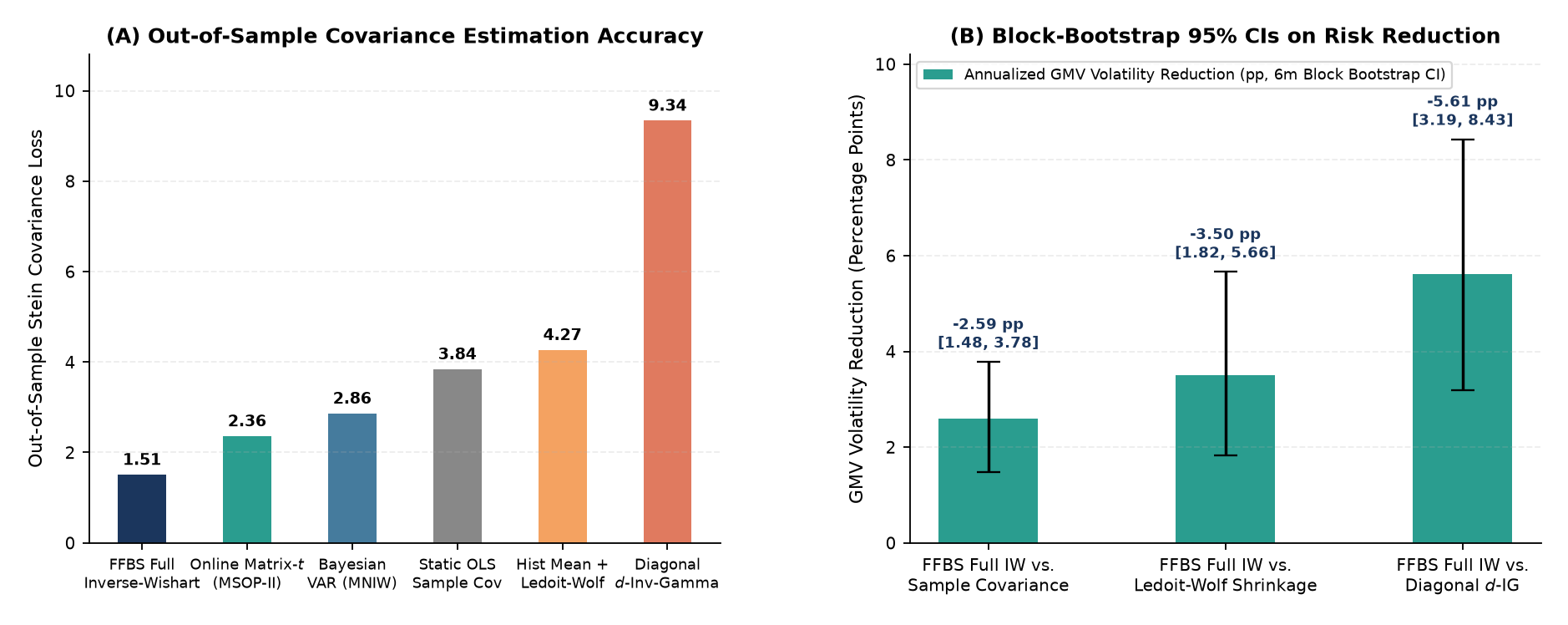
When the underlying series have a low signal-to-noise ratio in their conditional mean, Historical Mean + Ledoit-Wolf Shrinkage (\(\mathrm{RMSE} = 6.633\%\)), FFBS Full Inverse-Wishart (\(6.706\%\)), and Diagonal \(d\)-Inverse-Gamma (\(6.706\%\)) produce nearly identical point forecast RMSEs. However, modeling the full off-diagonal covariance matrix cuts Stein covariance loss from \(9.338\) (Diagonal) and \(4.267\) (Ledoit-Wolf) down to \(1.507\) (FFBS Full IW), improves the Multivariate Log Predictive Score from \(-18.210\) to \(-15.667\text{ nats}\), and significantly reduces Global Minimum-Variance (GMV) portfolio volatility by \(-2.59\text{ pp}\) vs. Sample Covariance, \(-3.50\text{ pp}\) vs. Ledoit-Wolf, and \(-5.61\text{ pp}\) vs. Diagonal \(d\)-IG under a 6-month moving-block bootstrap.

Model Architecture (120-Step Out-of-Sample Window)	Point RMSE	Multivariate LPS (nats)	Stein Cov Loss	Annualized GMV Vol
FFBS State-Space (Full Inverse-Wishart \(\boldsymbol{\Sigma}, \mathbf{Q}\))	\(6.706\%\)	\(-15.667\)	\(1.507\)	\(12.58\%\) (Best Risk)
Online Matrix-\(t\) Discount Filter (\(\mathrm{MSOP\text{-}II}, \delta=0.985\))	\(6.712\%\)	\(-15.842\)	\(2.359\)	\(13.34\%\) (\(94.31\%\) Cov)
Historical Mean + Ledoit-Wolf Shrinkage Covariance	\(6.633\%\) (Best Point)	\(-17.117\)	\(4.267\)	\(16.09\%\) (\(+3.50\text{ pp}\) Vol)
Diagonal \(d\)-Inverse-Gamma State-Space (Zero Off-Diag)	\(6.706\%\) (Same Mean)	\(-18.210\)	\(9.338\)	\(18.30\%\) (\(+5.61\text{ pp}\) Vol)

4 Exploring Further: Research Directions

Research Track	Core Question to Investigate	Tools & Methods
1. Riccati Convergence & Observability	How do the eigenvalues of \(\mathbf{F}\) and the rank of the observability matrix control the speed at which \(\mathbf{P}_{t\mid t}\) converges to \(\mathbf{P}_\infty\)?	Numerical Linear Algebra, Discrete Algebraic Riccati Equations
2. Adaptive Discount Factors in MSOP-II	Can we let the state discount factor \(\delta_t \in (0, 1)\) decrease automatically when a surprise innovation \(\mathbf{e}_t\) exceeds 3 standard deviations?	Online Bayesian Filtering, Dynamic Linear Models (West & Harrison, 1997)
3. LKJ Cholesky Priors vs. Inverse-Wishart	How does decomposing \(\boldsymbol{\Sigma} = \operatorname{diag}(\boldsymbol{\sigma})\,\boldsymbol{\Omega}\,\operatorname{diag}(\boldsymbol{\sigma})\) with an LKJ correlation prior compare to conjugate Inverse-Wishart as dimension \(d\) grows?	Cholesky Factorizations, High-Dimensional Covariance Shrinkage